Multiclass Image Classification Using Dense Neural Networks

Multiclass image classification categorizes an image into one of three or more classes. This tutorial demonstrates the concept using the MNIST handwritten digits dataset — 10 output classes (digits 0–9), 70,000 total images.

The MNIST Dataset

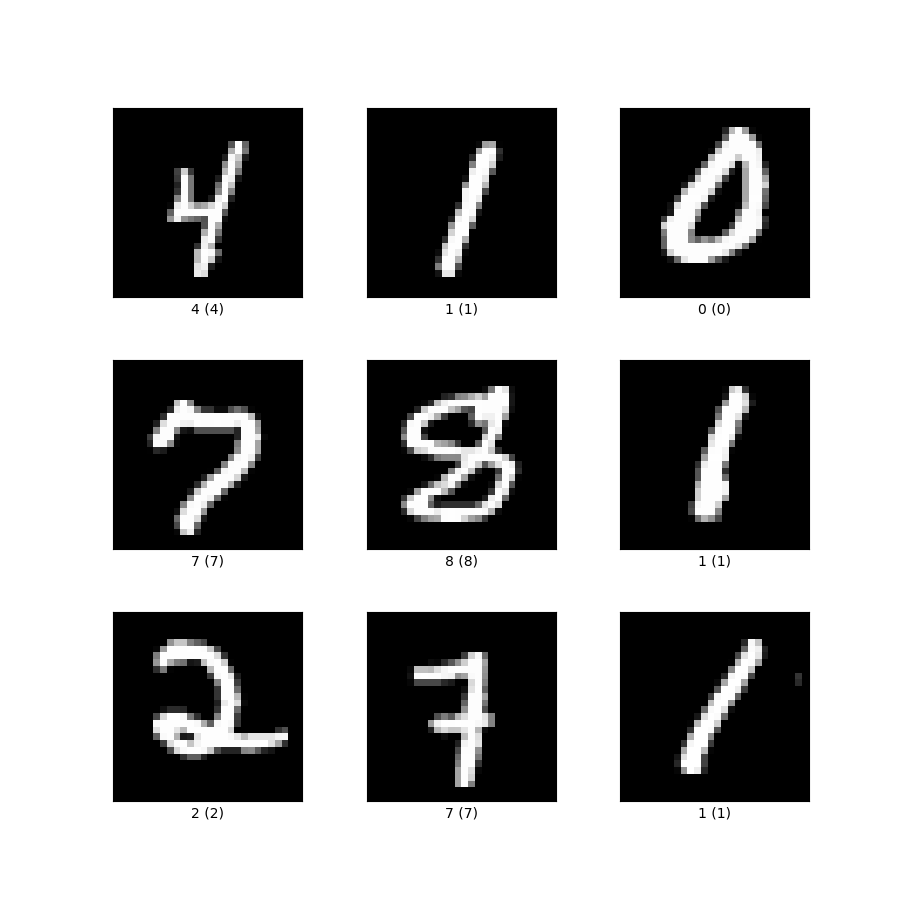
MNIST is the canonical benchmark for getting started with image classification. Each image is 28×28 pixels, grayscale, containing a single handwritten digit.

import tensorflow as tf
from tensorflow import keras
import numpy as np
import matplotlib.pyplot as plt

# Load dataset
(X_train, y_train), (X_test, y_test) = keras.datasets.mnist.load_data()

print(f"Training: {X_train.shape}")   # (60000, 28, 28)
print(f"Test:     {X_test.shape}")    # (10000, 28, 28)
print(f"Classes:  {sorted(set(y_train))}")  # [0, 1, 2, ..., 9]

# Visualize samples
fig, axes = plt.subplots(1, 5, figsize=(12, 3))
for i, ax in enumerate(axes):
    ax.imshow(X_train[i], cmap='gray')
    ax.set_title(f"Label: {y_train[i]}")
    ax.axis('off')
plt.show()

Preprocessing

Pixel values range 0–255. Normalize to [0, 1] for stable gradient descent, then flatten the 28×28 grid into a 784-element vector for Dense layers:

# Normalize
X_train = X_train.astype("float32") / 255.0
X_test  = X_test.astype("float32")  / 255.0

# Flatten 28×28 → 784
X_train = X_train.reshape(-1, 784)
X_test  = X_test.reshape(-1, 784)

print(X_train.shape)  # (60000, 784)

Building the Dense Neural Network

model = keras.Sequential([
    keras.layers.Dense(512, activation='relu', input_shape=(784,)),
    keras.layers.Dropout(0.2),
    keras.layers.Dense(256, activation='relu'),
    keras.layers.Dropout(0.2),
    keras.layers.Dense(10, activation='softmax'),  # 10 output classes
])

model.compile(
    optimizer='adam',
    loss='sparse_categorical_crossentropy',
    metrics=['accuracy']
)

model.summary()

Model: "sequential"
_________________________________________________________________
 Layer (type)           Output Shape         Param #
=================================================================
 dense (Dense)          (None, 512)          401,920
 dropout (Dropout)      (None, 512)          0
 dense_1 (Dense)        (None, 256)          131,328
 dropout_1 (Dropout)    (None, 256)          0
 dense_2 (Dense)        (None, 10)           2,570
=================================================================
Total params: 535,818

Architecture decisions:

• ReLU activation: avoids vanishing gradients in hidden layers, fast to compute
• Dropout (20%): randomly deactivates neurons during training — a strong regularizer
• Softmax output: converts raw logits into class probabilities summing to 1
• sparse_categorical_crossentropy: for integer class labels (no one-hot encoding needed)

Training

history = model.fit(
    X_train, y_train,
    epochs=10,
    batch_size=64,
    validation_split=0.1,
    verbose=1
)

Epoch 1/10 — loss: 0.2412, accuracy: 0.9282, val_accuracy: 0.9748
Epoch 5/10 — loss: 0.0823, accuracy: 0.9742, val_accuracy: 0.9791
Epoch 10/10 — loss: 0.0412, accuracy: 0.9872, val_accuracy: 0.9815

Evaluation

test_loss, test_accuracy = model.evaluate(X_test, y_test, verbose=0)
print(f"Test accuracy: {test_accuracy:.4f}")  # 0.9803

98.03% test accuracy with a simple 2-hidden-layer DNN in just 10 epochs.

Detailed Classification Report

from sklearn.metrics import classification_report

y_pred = np.argmax(model.predict(X_test), axis=1)
print(classification_report(y_test, y_pred))

              precision    recall  f1-score   support
           0       0.99      0.99      0.99       980
           1       0.99      0.99      0.99      1135
           2       0.98      0.98      0.98      1032
           3       0.98      0.98      0.98      1010
           4       0.98      0.98      0.98       982
           5       0.98      0.97      0.97       892
           6       0.98      0.99      0.98       958
           7       0.98      0.98      0.98      1028
           8       0.97      0.97      0.97       974
           9       0.98      0.97      0.97      1009
    accuracy                           0.98     10000

Balanced performance across all 10 digits — no class is significantly harder to classify.

Visualizing Predictions

predictions = model.predict(X_test[:10])

fig, axes = plt.subplots(2, 5, figsize=(12, 5))
for i, ax in enumerate(axes.flat):
    ax.imshow(X_test[i].reshape(28, 28), cmap='gray')
    pred = np.argmax(predictions[i])
    conf = predictions[i][pred]
    color = 'green' if pred == y_test[i] else 'red'
    ax.set_title(f"Pred: {pred} ({conf:.0%})", color=color)
    ax.axis('off')
plt.tight_layout()
plt.show()

Plotting the Loss Curve

plt.figure(figsize=(10, 4))
plt.plot(history.history['accuracy'], label='Train Accuracy')
plt.plot(history.history['val_accuracy'], label='Val Accuracy')
plt.xlabel('Epoch')
plt.ylabel('Accuracy')
plt.legend()
plt.title('Training vs Validation Accuracy')
plt.show()

Key Takeaways

• Dense networks work well for small, flat images like MNIST. For complex, high-resolution images, CNNs are far superior.
• Softmax + sparse_categorical_crossentropy is the standard recipe for multiclass classification.
• Dropout is a simple but effective regularizer — often all you need for small datasets.
• 98% test accuracy on MNIST is achievable with a basic DNN; CNNs push this to 99.7%+.
• Flatten first when using Dense layers on image data — preserve spatial structure only with Conv2D.

Next Steps

To go further:

1. Replace Dense layers with Conv2D + MaxPooling2D — expect 99%+ accuracy
2. Apply to a harder dataset: CIFAR-10 or Fashion-MNIST
3. Use data augmentation (ImageDataGenerator) to improve generalization